A Different Way of Looking at Returns

It would be nice if it were possible to trade a moving average cross. The problem with this is always that the data lags. It’s not possible to trade the current value of a moving average since it requires trading prices in the past. The advantage to doing so is that, due to the smoothing, forecasts are less noisy.

The good thing is than many moving averages are finite impulse response (FIR) filters, meaning they are the dot product of prices and weights. But can we compare the current price to a moving average? Well, yes, so long as it is an average in the future.

Implementation

The problem with log returns

is that they are very noisy. But let’s say we want to buy a position today and then sell it bit by bit over the next 7 days. What would that look like?

Using a filter like this, we can see the effective returns of such a strategy.

[1.000, -0.143, -0.143, -0.143, -0.143, -0.143, -0.143, -0.143]

This vector represents the amount of trading we will do at each time step. The position over time is given by the cumulative sum.

[1.000, 0.857, 0.714, 0.571, 0.429, 0.286, 0.143, 0.000]

You can see the position holdings are similar to buying on day one and then selling a little bit over the next days. You can be creative with this and say also buy over X, hold for Y days, and then sell over Z days. The world is your oyster.

Code

import ccxt
import pandas as pd
import numpy as np
from datetime import datetime
from plotly.subplots import make_subplots
from numpy.typing import NDArray

def make_mask(entry_len: int, wait_time: int, exit_len: int) -> NDArray[np.float64]:
    entry_ma_weights = [-1] * entry_len
    exit_ema_weights = [+1] * exit_len
    
    mask = np.array(list(np.divide(entry_ma_weights, np.abs(np.sum(entry_ma_weights))))
        + ([0] * wait_time) + 
                    list(np.divide(exit_ema_weights, np.abs(np.sum(exit_ema_weights)))))
    return mask

def rolling_dot(series: NDArray[np.float64], mask: NDArray[np.float64]) -> NDArray[np.float64]:
    n = len(mask)
    if n > len(series):
        raise ValueError("mask longer than series")

    # Construct sliding windows
    strided = np.lib.stride_tricks.sliding_window_view(series, n)
    # Each row is one window, so we do row-wise dot
    res = strided @ mask

    output = np.empty(len(series))
    output[-(len(mask)-1):] = np.nan
    output[:len(res)] = res
    return output

# Download historical daily data
exchange = ccxt.binance()
symbol = 'BTC/USDT'
timeframe = '1d'

# Fetch daily OHLCV (timestamp, open, high, low, close, volume)
ohlcv = exchange.fetch_ohlcv(symbol, timeframe=timeframe, limit=500)

# Convert to DataFrame
df = pd.DataFrame(ohlcv, columns=['timestamp', 'open', 'high', 'low', 'close', 'volume'])
df['timestamp'] = pd.to_datetime(df['timestamp'], unit='ms')
df.set_index('timestamp', inplace=True)

# compute returns
mask = make_mask(1, 0, 7)
df["convolved"] = rolling_dot(df["close"], mask) 

subtitles = [f"{symbol} Prices"]
nrows = len(subtitles)
specs = [[{"secondary_y": True}]] * nrows
fig = make_subplots(rows=nrows, cols=1, specs=specs, shared_xaxes=True, subplot_titles=subtitles)

# Add close price trace (primary y-axis)
fig.add_scatter(
    x=df.index, y=df['close'],
    name='Close Price',
    row=1,col=1,
    line=dict(color='blue')
)

# Add convolved signal (secondary y-axis)
fig.add_scatter(
    x=df.index, y=df['convolved'],
    name='Returns',
    line=dict(color='red', dash='dash'),
    row=1,col=1,
    secondary_y=True
)

fig.show()

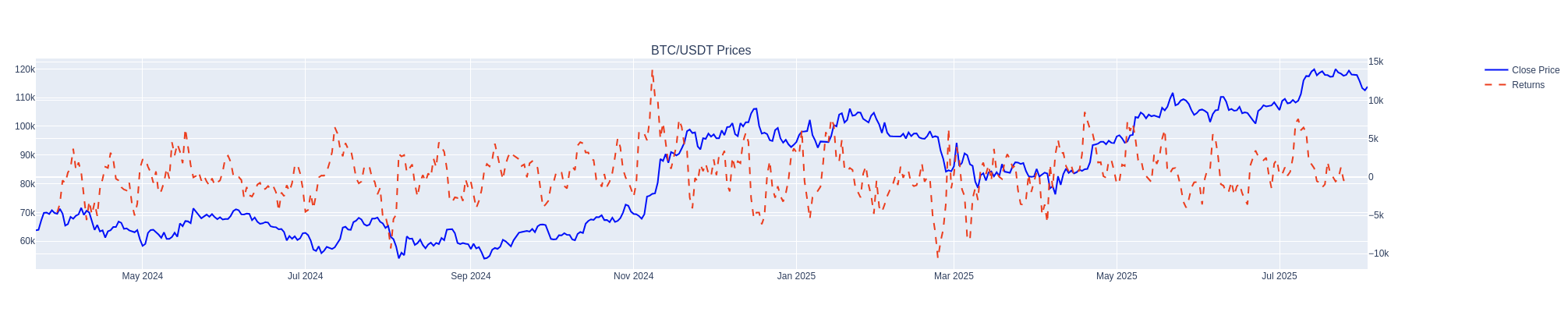
Strategy Returns

This is the resulting plot from the code above.

Variations on a Theme

Since this is easy to apply with any FIR-style filter, the position doesn’t need to be closed using an SMA. It is also easy to use triangle filters, an EMA, or whatever gives the strongest ability to forecast forward returns. The main advantage of this technique is that the noise of returns is reduced by using a smoothed exit. This means that the exit price is less dependent on chance, and it should be easier to find profitable opportunities.

It should also be noted that the autocorrelation of the returns should be avoided, as the returns themselves are not really known until much later. Forecasting should be done with signals independent of the return series.

Forecasting

The ultimate aim of this is to be able to predict returns using a set of features. This might be momentum, price extension, OI, funding, you name it. The hope is that using these returns as a dependent variable should make it much easier for machine learning to find something stable out of sample.

Trading

If you are holding positions for N periods, but forecasting every period, then how do you practically do that? Let’s say you have a filter that works over an 8-day period. Each period, you are rolling the position vector along one and then adding the position fixed vector. Then just check the current position and the first target position value, and trade the difference.

position = np.array([1.000, 0.857, 0.714, 0.571, 0.429, 0.286, 0.143, 0.000])

# Create a vector of length 14 to accumulate contributions
agg = np.zeros(14)

# Apply the position vector starting on days 0 to 6
for i in range(7):
    agg[i:i+8] += position

# Display the result
np.set_printoptions(precision=3, suppress=True)
print(agg)

Final Note

This was just a quick article about something I thought others might find helpful in case they were struggling with predicting returns. There is an old adage that if you get a good entry, the exit should be easy. This is a variation on that theme. As always, I appreciate the feedback, so please let me know if you found this useful.