Alpha Decay

I have been thinking a lot about reinforcement learning since it seems to be an interesting technique for creating trading strategies. Reinforcement learning is a simple idea and can be implemented in different ways from Q learning, actor-critic models and other deep learning techniques. The general idea is, given a set of actions A, there is a value function V which gives the quality of each action given the state S. A discrete action set is useful for micro-structure based execution algorithms where in essence there are two options, have an order at touch or pull the order. Given the order’s queue position, order book shape, flow toxicity, exchange latency and other state variables we can decide the best action to take. The part I am currently wondering about is how to properly calculate a value function. I think for optimising execution algorithms the implementation shortfall can be used. The implementation shortfall is the difference between the final executed price and a benchmark. Common benchmarks include the mid-price at time of order or volume-weighted average price (VWAP). The VWAP is better because it takes into account the cost of liquidity which is variable over time and order size. One issue I have still to work out is that each fill might be associated with a chain of different actions. An order might be moved multiple times before its filled, and might be filled over different price levels. In a perfect world, there would be a 1:1 mapping between action and implementation shortfall but it would seem there needs to be a different solution to this problem. I have read this is an issue in teaching AIs to play games as goals such as “killing a boss” required chaining different actions together.

Reinforcement learning allows the value of an order’s queue position to be implicitly included in the value function. There is an opportunity cost associated with moving an order since every time an order is amending the queue position is lost. Properly accounting for opportunity cost is difficult to accomplish with other techniques. A trained RL model should learn to move orders sparingly since a model that has a high value associated with the pull order action is likely to have a lower total reward compared with a version which uses this action very sparingly.

Using reinforcement learning for risk-taking trading strategies is more complicated than simple execution strategies due to the value function being more complicated. Trading strategies are assessed using measures such as profit factor, compound annual growth rate (CAGR), Sharpe ratio which uses the whole trading history. This is an issue with the bellman equation that reinforcement learning uses since there needs to be a mapping between the quality of action given the state and the action. This is where some other measures may be of use.

Alpha Decay

Another technique that came to mind is called alpha decay charts. This can be used to work out the optimal exit timing for a trade and also a possible exit strategy depending on return skew. The price distribution post fill is ideally skewed and has a positive mean. Mean reversion trading signals also often only work for a certain amount of time. Since they are cyclical and the cycle half-life means that after a long time if the exits have not been hit likely the cycle will be against the direction of the trade.

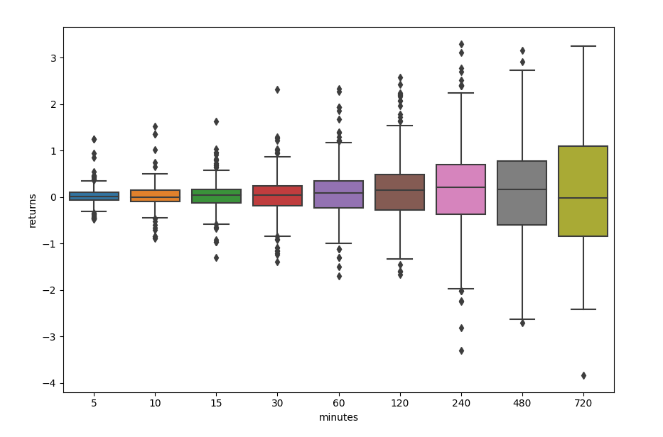
The plot shows the distribution of returns at different time points post a trade. The mean value can be seen to increase over time until about 4 hours where they decrease. It can also be seen that the skew is high immediately after a trade suggesting the signal also has good market timing. A four hour holding time for this signal looks like it would be advantageous for this signal.

The code of the plot is as follows

import numpy as np
import pandas as pd
import seaborn as sns
import matplotlib.pyplot as plt

alpha_df = pd.DataFrame()
trade_times = trade_df.index
trade_price = list(trade_df.price)
for offset in [5, 10, 15, 30, 60, 120, 240]:
    # calculate future price
    fut_price = price_df.price.asof(trade_times + timedelta(minutes=offset))

    # calculate returns
    returns = 100*np.log(np.divide(fut_price, trade_price))
    returns *= list(np.sign(trade_df.fill_qty)) # change return sign for long/short

    # build results dataframe
    tmp_df = pd.DataFrame(zip(returns, [offset]*len(returns)), columns=["price", "offset"])
    alpha_df = pd.concat([alpha_df, tmp_df])

# plot alpha curve
plt.figure()
sns.boxplot(data=alpha_df, x="offset", y='price', orient='v')
plt.ylabel("returns")
plt.xlabel("minutes")
plt.figure()

Producing the plot is simple with pandas and simply requires looking up the relevant prices at different points after the fill or signal.

Profit factor

Alpha decay charts are useful for understanding a signal’s performance however what is needed is a value function for an individual fill. I was reading a book by Timothy Masters called Testing and Tuning Market Trading Systems. In the book, profit factor is discussed as a method of assessing signal quality. Profit factor is a simple calculation and

The issue with the profit factor calculation in most trading software is that it takes the open and close price of each round trip order. The pnl per trade is then calculated as direction * (close price - open price). The issue with this is that the distribution of returns over the lifetime of the trade is lost. It is better to have a trade that doesn’t have any drawdown and goes directly to the profit target compared to one that went deep into drawdown before becoming profitable. Masters solution to this is clever in its simplicity. The profit factor is calculated over the life of the trade sampled at regular intervals. This means that the distribution of returns over the lifetime of a trade can be measured and in the case of a profitable trade with a large drawdown leads to a lower profit factor.

It is interesting to plot the master’s style profit factor against signal quantiles. In the case of a good signal, it is often the case that the upper/lower tails of the signal show a significantly better profit factor. This parallels the classification work I have done in that only 20% of cases can be classified with enough precision to justify their inclusion into a strategy. A strategy with a high master’s style profit factor will not only be profitable but will also have good market timing leading to lower drawdowns. There is the added benefit that it can be applied to individual fills. There are effectively two hyperparameters, the sampling interval and the time over which the signal is to be assessed.

Summary

I think the master’s style profit factor could be used as a basis for the value function in RL because it gives a measure of both the profitability of a trade but also the market timing. It is also simple and computationally efficient. The alpha decay chart gives more overall information, but it is not clear to me how this could be converted to a single measure that can be used to evaluate the performance of individual actions.

more to follow…