I recently came across tr8dr.github.io and specifically this post. I only recently found this site and its older version even though it has been around for a long time. I am a big fan of this blog and after reading the post was wondering if the technique could be used to train an online labeller using an HMM model. The idea is to use the labeller offline to generate 3 return classifications, trend up, down and no trend. Then by looking at the distributions of returns in each of the classes it should be possible to determine online which of the 3 states we are most likely to be in. My hypothesis is that the 3 classes can be modelled as two skew-normal distributions for trend up/down and a normal distribution for the neutral market. These distributions would be fitted separately to the training of the transition matrix for the hidden markov model (HMM). The then fitted HMM would be ready to be used online with new data it has not seen before… at least that is the plan!

Using the labeler that can be found here. I applied this labeller to 5 minute BTCUSD closes.

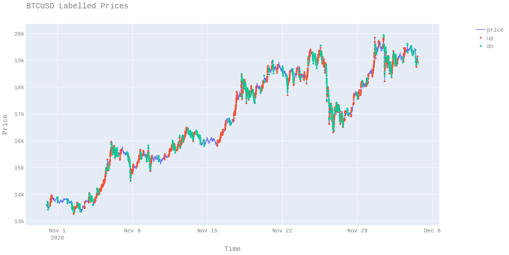
The parameters for the labeller are 100 basis points and 10 inactive bars.

from tseries_patterns import AmplitudeBasedLabeler
labeler = AmplitudeBasedLabeler(minamp=100, Tinactive=10)

Unconditional Distributions

We can see from the plot the labeller does a good job of identifying areas where the market is trending. The second interesting observation is that there is a lot of auto-correlation between the states. It is the stickiness of these states which is what we will be trying to make money from. If it is possible to successfully identify the market state then the assumptions are that the market is more likely to stay in that state.

An offline labeller is only so useful in the real world. What we want is something that can tell us real-time what type of market we are in. These distributions are what allows us to use a hidden markov model (HMM) as an online labeller.

HMM Fitting

As a refresher to how HMMs work, if we assume we have a gaussian HMM then each distribution gives us the ability to calculate the unconditional probability of the observation assuming the state is known.

where \(\phi\) is a normal pdf. What we want to know is \(Pr(S_t | x_t)\) meaning what market state are we in given the most recent return? The way an HMM works is to compute \(Pr(S_t | x, S_{t-1})\) by computing or specifically given the previous state of the market and the unconditional probability of the observation what is the most likely current state. For more information about HMMs, I can recommend the book Hidden Markov Models for Time Series: An Introduction Using R.

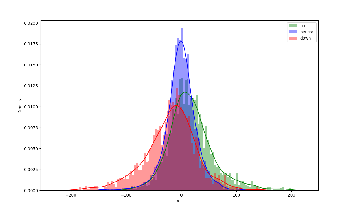
Fitting distributions is easy in python and the code for this can be found below. I have assumed the up and down distributions are skew-normal and the sideways distribution is normal. I did not test the AIC or BIC of the fit but I have enough confidence from visual inspection alone that this is better than using a normal distribution for all states.

df["ret"] = np.log(df.price / df.price.shift(+1))
up_dist = skewnorm.fit(is_df[is_df["label"] == +1]["ret"])
neutral_dist = norm.fit(is_df[is_df["label"] == 0]["ret"])
dn_dist = skewnorm.fit(is_df[is_df["label"] == -1]["ret"])

[2.0001465928288162, -0.0012649549909783588, 0.0031376480456382326]
[-1.5579584949819384e-05, 0.0015993374693992941]
[-2.0632362428891016, 0.0016759065121076458, 0.003912295938373958]

Fitting an HMM

Given we have this assumption in regards to the return distribution in each state can we fit an HMM to be used online? Using the hmm learn library this is easy to do even if the emission distribution is non-gaussian. By overriding the HMM base class to be able to calculate the log-likelihood for the various distributions allows the data to be easily fit.

from scipy.stats import skewnorm, norm
from hmmlearn.base import _BaseHMM

class CustomSkewHMM(_BaseHMM):
    def __init__(self, params, **kwargs) :
        self.dists = [
            skewnorm(params[0], params[1], params[2]),
            norm(0, params[3]),
            skewnorm(params[4], params[5], params[6]),
        ]

        super().__init__(**kwargs)

    def _compute_log_likelihood(self, X) :
        res = np.zeros((X.shape[1], len(self.dists)))
        for i, density in enumerate(self.dists):
            res[:, i] = density.logpdf(X)
        return res

To fit the data can then be done simply via the following commands.

    params = [2.0001465928288162, -0.0012649549909783588, 0.0031376480456382326,
              0.0015993374693992941,
              -2.0632362428891016, 0.0016759065121076458, 0.003912295938373958]
    hmm = CustomSkewHMM(params=params)
    hmm.fit(X=returns)

The results of the fit are as follows

print(hmm.transmat_)
[[0.93346208 0.05151349 0.01502443]
 [0.03678946 0.96321054 0.        ]
 [0.16128029 0.         0.83871971]]

We can see that the diagonal matrix are close to one. This means that the market tends to stay in the same state. This can also be corroborated via the confusion matrix for the in-sample labels.

confusion_matrix(is_df["label"][1:], is_df["label"][:-1])
[[1943   78   86]
 [  66 2093   99]
 [  98   88 2447]]

What is also interesting from the fit is that it suggests the market is more likely to go from a down market to an up market compared to a sideways market. We are also 3 times more likely to go from an upmarket to a sideways market.

Online classification

The true test is whether the calibrated HMM can correctly classify the market state online. To do this we will fit the out of sample data and compare those with the labelled results from the offline labeller.

If we look at the confusion matrix of the known out of sample labels

[[ 460   46  107]
 [  52 1121   27]
 [ 100   34   52]]

It seems like in the out of sample data the transition matrix should be quite different. It looks like a tendency to trade sideways but rarely does there seem to be a down market.

The estimated states from HMM however are not very close to the actual labels.

print(confusion_matrix(y_true=oos_df["label"], y_pred=hmm_states))

[[187 278  73]
 [118 464  33]
 [308 459  80]]

print(classification_report(y_true=oos_df["label"], y_pred=hmm_states))

              precision    recall  f1-score   support
        -1.0       0.31      0.35      0.32       538
         0.0       0.39      0.75      0.51       615
         1.0       0.43      0.09      0.15       847
    accuracy                           0.37      2000
   macro avg       0.37      0.40      0.33      2000
weighted avg       0.38      0.37      0.31      2000

I can only presume the reason for this is that the estimated parameters for the unconditional distributions are not stable. It would seem that the state persistence is stable through time however the main reason I suspect for out of sample performance is bad is if the parameters for the unconditional models differ by a lot. This needs more investigating.