Return Classification

Today BTC finally broke the all-time high and seems to be holding well above 20k USD. At this point, all bets are off as to where the bull market will end. Technical analysis is not very useful when market profile or historic prices can not be used. The historical precedent is 10x gains which would mean targets of 100k are not unreasonable (some investment banks such as Morgan Stanley have price targets of 160-250k, Plan B has a S2F flow model target of 288k). It seems like the dynamics of the market have also changed recently. There has been a lot of resistance to bitcoin as a store of value from traditional money managers. This is mostly due to its volatility, but the volatility will be lower when there are more people actively investing in it rather than the incredible amount of speculation that has been taking place. Recently there have been large asset managers public announcing their purchase of 100s of millions of dollars of bitcoin. These amounts are well above the mining capacity of the system to its effect it to severely limit supply pushing prices up. Given the debasement of fiat Gresham’s law suggests that bitcoin will likely be stockpiled as fiat eventually becomes worthless.

Classification Models

When using machine learning classifiers for trading it’s important to note that the loss function, is quite different from many other domains. If we consider the detection of COVID-19 cases it is better to have high recall, if there is an acceptable loss in precision since its better to have a person tested twice than to have a person unknowingly spreading the virus. The cost of a false positive is thus less than a false negative.

In the case of trading, this is the complete opposite.

from sklearn.ensemble import RandomForestClassifier, AdaBoostClassifier
from sklearn.metrics import confusion_matrix

cle = RandomForestClassifier(max_depth=3, n_estimators=10, max_features=3)
clf = AdaBoostClassifier(base_estimator=cle, n_estimators=100, learning_rate=0.01)
clf.fit(x_train, y_train)

predict_actual = clf.predict(x_test)
print(confusion_matrix(y_test, predict_actual))

[[ 242 1031]
 [ 201 1114]]

The rows of the confusion matrix are the actual outcome, and the columns are the predicted values. The out of sample prediction quality is bad. The mean of the signal adjusted returns is positive, so the model is simply predicting the return will be mostly positive. We can see out of sample it is almost always wrong.

The issue is the loss function for trading is heavily skewed towards accuracy especially when transaction costs and fees are taken into account. A false positive is a losing trade, whereas a false negative is missing a trade that would have been profitable. It is thus preferable to aim for higher accuracy over recall.

decision_function = clf.decision_function(x_test)
precision, recall, treshold = precision_recall_curve(y_test, decision_function)

# Plot the output.
plt.figure()
plt.plot(treshold, precision[:-1], c='r', label='PRECISION')
plt.plot(treshold, recall[:-1], c='b', label='RECALL')
plt.grid()
plt.legend()
plt.title('Precision-Recall Curve')
plt.show()

Looking at the classification report we can see the performance of the standard model is no better than flipping a coin.

The standard classification report returns the value with an optimal F1 score. By plotting the precision-recall curve it is pretty easy to see this point as the cross over of the precision and recall lines.

              precision    recall  f1-score   support
           0       0.52      0.35      0.42      1491
           1       0.52      0.69      0.59      1529
    accuracy                           0.52      3020
   macro avg       0.52      0.52      0.51      3020
weighted avg       0.52      0.52      0.51      3020

Some classifiers in scikit-learn make it possible to output the classification score. Using this score allows the precision-recall curve to be plotted. This chart gives the ability to examine the trade-off between accuracy and recall.

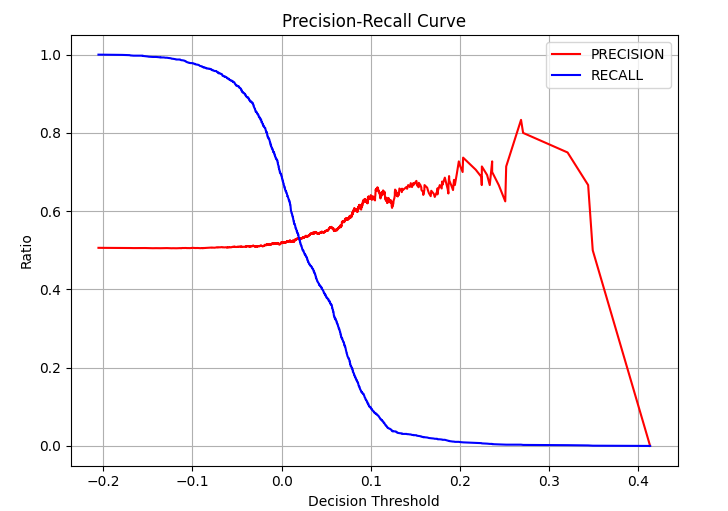
By changing the decision threshold of the classifier the accuracy increases. For a small increase in accuracy, the recall is significantly reduced. It is possible to use various trading loss functions across the different thresholds to work out the best one to use for trading. The loss functions include, sum, sharpe, profit factor, pnl/max draw down etc. In the graph below sum(pnl) is used, however this technique is applicable irrespective of which trading loss function is used.

def calc_pnl_curve(returns, score, nsamples=100, loss=np.sum):
    """
    :param returns: out of sample trading returns
    :param score: classifier score function
    :param nsamples: number of threshold samples required
    :param loss: trading loss function
    """
    pnls, trade_counts = [], []
    thresholds = np.linspace(np.min(score), np.max(score), nsamples)
    for threshold in thresholds:
        rets = returns[score > threshold]
        trade_counts.append(len(rets))
        pnls.append(loss(rets))
    return thresholds, trade_counts, pnls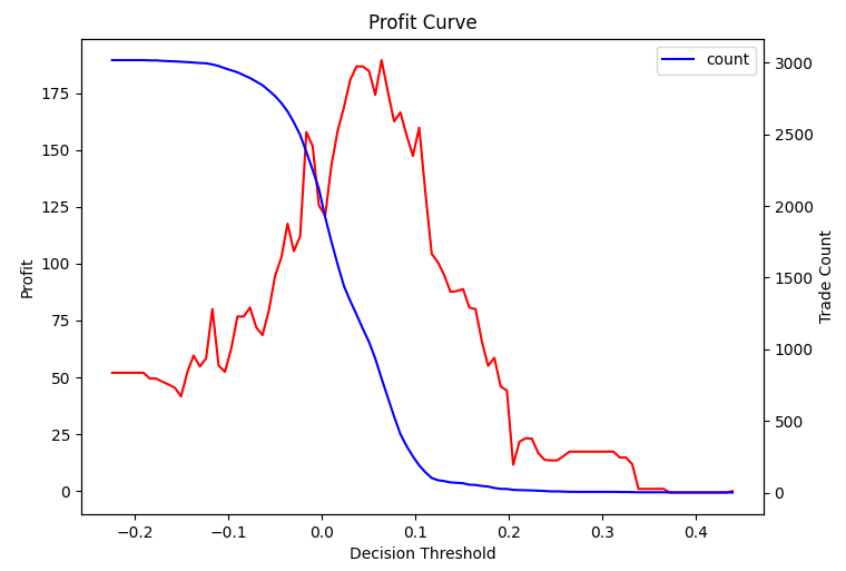

If all trades are included, the total profits are lower than if the best are cherry-picked. If the threshold is too high then there not many trading opportunities, lowering profits. There is a Goldilocks zone in between where expected profits are maximised. From the profit curve, the optimal threshold is about 0.08. This gives a precision of about 60% but a recall of about 20%. This is a better way of choosing the threshold compared to using the F1 score of the standard fits within scikit-learn.

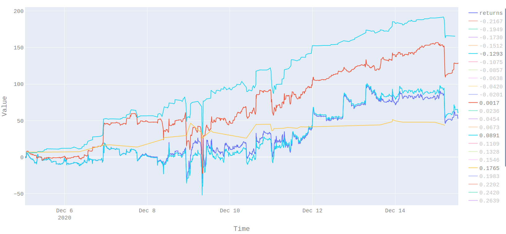
Out of Sample Returns

As a rough inspection of the out of sample returns it is possible to see the effect of the model choice. A threshold of 0.0891 gives a profit of three times the return of just betting on ever trade. It would seem from visual inspection that the risk-adjusted return of the classification model is also better.

Next Steps

The analysis looks promising and seems to be ready to be integrated into a backtest.

• Update the live model to use a classifier.
• Backtest recent data to check profitability