MCMC for Return Distributions
How do you know if a return distribution is skewed? The empiricist method is to fit the data to a normal and skew-normal distribution and to compare the AIC or BIC of each fit. I would like to present an alternative that is more powerful and is also useful for giving confidence intervals to estimate the quality of fit of each parameter. This is especially useful for computing correlation matrices since most techniques only give point estimations and not parameter distributions.
Markov chain monte carlo (MCMC) is an alternative method for estimating model parameters and often gives better interpretability compared with methods that rely specifically on maximum likelihood estimation (MLE) or maximum a posteriori (MAP) estimation. Libraries such as pymc3 make it simple to do MCMC in python.
In the case of the skew normal its 3 parameters, \(\mu\), \(\sigma\) and \(\alpha\)
\[f(x | \mu, \sigma, \alpha) = 2\Phi ((x-\mu) \sqrt{\tau} \alpha) \phi(x,\mu, \tau)\]What mcmc practically does is sample from distributions for each of the parameters that are unconditional and user-specified. Then given the difference in the likelihood of the current value, and the new value, the new parameters are either accepted or rejected with a probability proportional to its improvement in the likelihood. This is done repeatedly in what is known as a chain. The chain should eventually converge to the correct value of the parameter. What is an added benefit is that the chain can deviate from the optimal value. The range of this deviation can be interpreted as a confidence interval. What we would like to know is the parameter distribution however estimating the join probability \(f(\mu, \sigma, \alpha | x)\) from the data is difficult, however the alternative \(f(x | \mu, \sigma, \alpha)\) is simple to estimate and simulate via standard distributions in this case via a skew-normal distribution. The only thing needed to be decided is what unconditional distribution the parameters might take. In the case of the skew-normal
\[\mu \in \mathbb{R}\] \[\sigma, \alpha \in \mathbb{R}_{>0}\]\(\mu\) is estimated to follow a standard normal distribution, \(\sigma\) follows a beta distribution which ensures its positiveness and \(\alpha\) follows a half-normal distribution since its also positive but not bound below one. The goal is to choose a distribution that has a lot of the density around the correct parameter value this can be done via a trial and error or other empirical approaches can be taken for a starting guess.
This is the code for fitting a skew-normal distribution to our return data using pymc3.
import pymc3 as pm

with pm.Model() as model:
    mu = pm.Normal("mu", mu=0, tau=1)
    alpha = pm.HalfNormal('alpha', sigma=1.)
    sigma = pm.Beta('sigma', alpha=1., beta=3.)
    y = pm.SkewNormal('y', mu=mu, sigma=sigma, alpha=alpha, observed=data)
    trace = pm.sample(10000, chains=10, cores=10, random_seed=42, progressbar=True)
    burned_trace = trace[2000:]
pm.traceplot(trace)
The results from running this code on our bitcoin up leg return distributions are.
- \(\mu\): -0.00165
- \(\sigma\): +0.00325
- \(\alpha\): +1.44022
However, these numbers are not that useful since we could have just gotten them from scipy.stats.skew-normal.fit(data). The interesting information is in the trace distributions. Notice we use burned_trace and not trace, the reason for this is that the first values in the monte carlo simulation are likely to be a long way from the correct values. For this reason, the first x samples are often discarded to remove their influence from the final values.
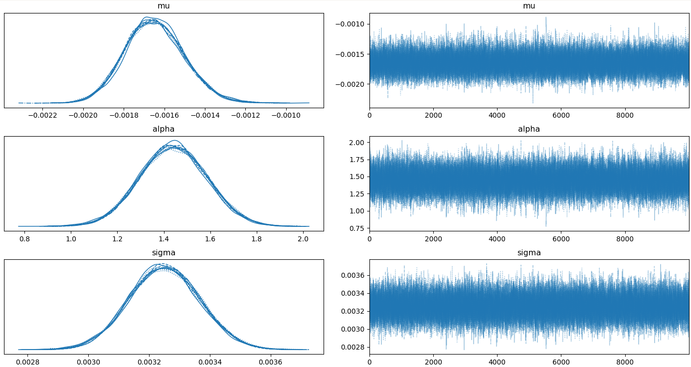
We can see the confidence interval from the trace plots.
import numpy as np
print(np.percentile(burned_trace['mu'], [2.5,97.5]))
> [-0.00192294 -0.00134684]
print(np.percentile(burned_trace['sigma'], [2.5,97.5]))
> [0.00302327 0.00348046]
print(np.percentile(burned_trace['alpha'], [2.5,97.5]))
> [1.15570184 1.72671967]
The 5% two-tail confidence interval for alpha is [1.15570184 1.72671967] which means we can reject the null hypothesis of H0: \(\alpha\) = 0.
Follow up
MCMC is really powerful and can be used to estimate complicated stochasitc models such as:
- Heston model:
- Vasicek model: \(dr_t = \theta (\mu - r_t) dt + \sigma dW_t\)
- CIR model: \(dr_t = \theta (\mu - r_t) dt + \sigma \sqrt{r_t} dW_t\)
- Chen model:
which are hard to estimate via other means.
There is also a close association between particle filters and MCMC. Particle filters can be used online to estimate these models. To do this however we need to know the parameters of the evolution process and also the model errors. MCMC can be used offline to configure the parameters of a particle filter and then that filter be used online to make predictions. I will at some point write a post about these topics.