In 2014, I went to talk by a collection of asset managers hosted by Bloomberg. This is one of the nice perks of having a Bloomberg terminal. The speakers were large asset managers and not short term traders; their conclusion was to make money you need to be looking at quarterly returns since at lower time frames the noise is too significant. They were trading billions of dollars so likely their opinion was skewed by practical issues associated with execution fees and slippage. Managing that amount of money is a different game due to needing to hide your intentions while simultaneously being filled.

At this talk, the head of gold analysis at HSBC London remarked,

When volatility is high market make, when it is low follow the trend

In my opinion, the statement is correct, but I take issue with the term “volatility”. Is all volatility the same? Reflecting on the statement, I think that “when noise is high market make when it is low follow the trend” is more accurate. Markets move, but not all moves are equal. Some moves are directional and do not mean-revert, some have a disproportionate amount of noise.

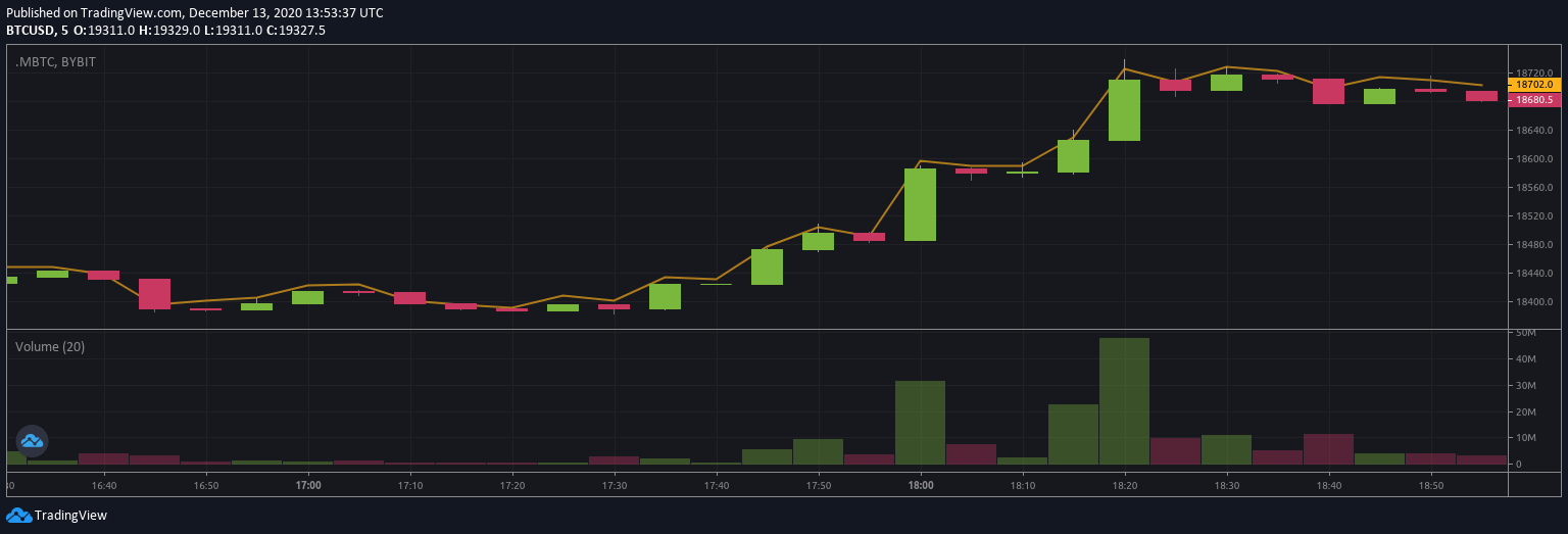
Directional Market Move

Noisy Market Move

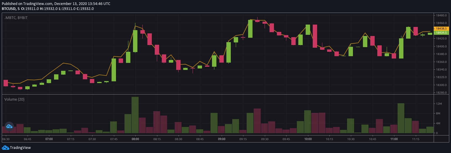
My issue with volatility measures is that in both cases, volatility is high. These, however, are completely different ‘styles’ of market and should be approached as such. Thus just looking at volatility alone is not enough.

It would be much more profitable to follow the trend in market 1 whereas in market 2 there would likely be more profitable to market make. Financial time-series are fractal in nature, so a non-trending noisy market in one timeframe is a trendy market in another. For now, I would like to put this aside, since I think that is more related to model selection. This post aims to talk about estimating market noise and trying to classify the market-style conditional on a specific timeframe.

Bayesian Market Making

The papers about Bayesian Market-Making and Optimal Sequential Market-Making cover the same topic.

The paper was interesting to me since it is a form of reinforcement learning. The proposition is that market making is an exploratory as well as exploitatory problem. The goal is to estimate the correct fair price as quickly as possible and to then trade as much volume as possible around it before it moves to a price level. By decreasing your spread you can pay for information. When orders are filled, the spread, as well as the time it took for that order to be filled, could be used to update the prior distribution for the fair price.

The paper also discusses the information disadvantage of the market maker that I have not seen talked about elsewhere.

The market maker’s state is characterized by a Gaussian belief for the value of the market \(V: N(\mu t, \sigma^2_t)\). The trader signal is assumed to be normally distributed around V, so \(s∼N(V, σ^2_\epsilon)\). The main relevant parameter(see [Das and Magdon-Ismail2008]) is the information disadvantage of the market maker, \(\rho_t = \sigma_t/ \sigma_\epsilon\), the ratio of the uncertainties of the market maker and trader.

In essence, the noise volatility needs to be estimated separately to the volatility of the price process. Later in the paper, they mention empirical experiments showing if the informational disadvantage \(\rho_t = \sigma_t/ \sigma_\epsilon\) is too high (>3) then market-making stops being profitable. When this is the case the profit from the noise (mean reversion) does not compensate for the uncertainty of the true price.

To update the statement from the first paragraph

when \(\rho\) is low market make, when it is high follow the trend

Likely in the application, this should use a smooth transition between states rather than a single cut off value. It is shown by simulation that the relationship between profits and \(\rho\) is non-linear and pnl decrease significantly beyond a \(\rho\) value of 2.5.

Trading Application

The strategy I am running a mean reversion strategy on cryptos that is in essence a market marker. It estimates a mid-price and then positions itself with the expectation that the future mean price is likely to be the forecasting average price. This strategy is more likely to make money in a noisy market non-trending market. I plan to predict the strategy pnl using estimates of \(\rho\) and other factors and then use this prediction to scale the live risk. In favourable market conditions, it should over-perform and in trending markets ideally, it should stay out and wait.

Market profiles

Market profiling is a technique for finding price areas that may have significance in the future. Simple implementations of the market profile simply segment time uniformly and plot a histogram of volume for each time block. Volume tends to coalesce around a certain price and also tends to behave differently when the market returns to a price where a lot of volume previously traded. Market profiles are useful for entry points and exit points from trades. If there has previously been a lot of trading in a certain price area it is more likely that the price will reverse again at the same price due to un-executed orders that remain in the market.

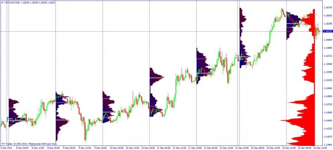
Looking at a plot of the market profile from a simple time-based implementation its possible to see that the market trading around a mean and then jumping to a new mean. Better methods of producing market profiles involve segmenting the data so that the volume distributions are as disjoint as possible. The market profile suggests a similar market dynamic which is counter to the idea that prices follow a continuous distribution. Even if the price arguably does, the volume certainly does not. There are however a set of stochastic processes that deal with these jumps.

Jump Diffusions

The stochastic differential equation (SDE) for Brownian motion is

\[\frac{dS_t}{S_t} = rdt + \sigma dW_t\]

In this case there is only one volatility \(dW_t\) which is in essence the assumption when volatility is calculated on returns via the standard deviation \(\sigma ={\sqrt {\operatorname {E} \left[(X-\mu )^{2}\right]}}\)

This is however too simple and can be extended to the Merton jump diffusion process,

\[\frac{dS_t}{S_t}=(r−\lambda \bar{k})dt+ \sigma dW_t+kdq_t\]

The jump event is governed by a compound Poisson process \(q_t\) with intensity \(\lambda\), where k denotes the magnitude of the random jump.

The distribution of k obeys

\[ln(1+k) \sim N(\gamma, \delta^2)\]

The jump-diffusion is an extension of the standard Brownian motion process where at each point in time there could be a jump with a random magnitude. There is thus 3 sources of randomness \(dW_t\), \(dq_t\) and \(\lambda\). I was thinking that this could explain the thinking behind noise volatility vs price process volatility. The noise could be regarded as \(dW_t\) whereas the price process volatility is related to \(dq_t\) and \(\lambda\).

Next Steps

I want to spend more time working on market profiles. I plan to use MCMC and Dirichlet Processes to find an optimal segmentation for the market prices. I recently learnt about the earth movers distance that could be useful for computing a set of Gaussian mixtures that are maximally disjoint. I think this is an aside however from trying to use an online particle filter to try to estimate the parameters of a jump-diffusion process. Having the market profile correctly computed would mean it is possible to check if \(dq_t\) and \(\lambda\) are constant or time-varying. I assume that they are not in clock time but might be in volume time. This assumption will have to be tested empirically. What all this is done it will be possible to have an online estimated for \(\rho\) and to use the informational disadvantage in trading strategies.